Selection of Tantalum Capacitors from Failure Cases: True Performance and Alternatives of ECS-F1HE475K in High Voltage Transients

In a field failure analysis of industrial power modules, engineers discovered that Panasonic ECS-F1HE475K (4.7µF/50V) tantalum capacitors on multiple boards suffered short-circuit failures at the moment of system power-on. This article provides an in-depth analysis of their limitations and offers reliable replacement solutions based on the failure mechanisms. In-depth Review of Failure Case: What Happened on Site? This case originated from a 24V to 5V DC/DC power module supplying a servo driver. During burn-in testing after mass production, some modules experienced no-output failures upon startup, with a failure rate of approximately 0.5%. Failure Background: Application Scenario and Circuit Environment Analysis The failed ECS-F1HE475K was located at the input filter position of the module, directly connected in parallel across the 24V input. Circuit analysis showed that the front end of the system lacked effective soft-start or surge suppression circuits. In actual factory environments, due to the starting and stopping of high-power equipment, input ports are highly susceptible to coupling high-voltage spikes with widths of tens of microseconds and amplitudes far exceeding the rated voltage. Failure Phenomenon: Physical Damage under EM and Root Cause Decapsulation and Scanning Electron Microscopy (SEM) analysis of the failed capacitors revealed obvious breakdown channels between the tantalum anode block and the manganese dioxide cathode layer, a typical "avalanche" failure. The root cause points to irreversible lattice structure changes in the manganese dioxide cathode when the capacitor is subjected to transient overvoltages far exceeding its rated surge voltage capability, leading to a sharp increase in leakage current and ultimate thermal breakdown. ECS-F1HE475K Datasheet Interpretation and "Ideal" Discrepancy Rated Voltage 50V Actual Surge Withstand ~35V Recommended Operating Voltage 25V Re-evaluating Key Parameters: Rated Voltage, Surge Voltage, and ESR Reviewing the official manual for this model, a nominal 50V rating for a 24V circuit seems to provide more than double the voltage margin. However, the transient surge voltage of manganese dioxide cathode tantalum capacitors is typically only 70% of the rated voltage. This means a 50V rated model may actually withstand a surge voltage of only 35V. Additionally, while low ESR is beneficial for filtering, it can lead to higher instantaneous inrush currents during transient overvoltages. "Shortcomings" Not Explicitly Stated in Data Sheets: Tolerance to Transient Overvoltage Data sheets are usually based on steady-state test conditions, whereas dynamic stresses such as voltage transients, reverse peaks, and ringing in real applications are far more severe. Manuals often lack detailed curves regarding the tolerance for repetitive pulse overvoltages, which is precisely the root cause of many selection errors. Tantalum Capacitor Failure Mechanism: Why are High-Voltage Transients the "Killer"? The "Avalanche" Effect of Manganese Dioxide Cathodes The semiconductor characteristics of manganese dioxide (MnO₂) dictate that its resistivity drops exponentially as the electric field increases. Transient overvoltages trigger a surge in local current density, generating Joule heat and forming positive feedback, which ultimately leads to localized thermal runaway within microseconds. Voltage Derating: Gap Between Theory and Practice The industry generally recommends a 50% voltage derating. However, facing high-frequency, high-energy transient shocks, even derating to 35V may be insufficient. In environments with significant surges, it is recommended to limit the operating voltage to 30%-40% of the rated value. Core Principles for Tantalum Capacitor Selection under High-Voltage Transient Conditions 1 Principle One: Selection Based on Voltage Derating Ratio Core Principle: The maximum possible transient peak voltage in the circuit (including all ringing and spikes) must be lower than the capacitor's rated surge voltage. Precise measurement with an oscilloscope is recommended. 2 Principle Two: Series Resistance and Circuit Impedance Requirements Connecting a small current-limiting resistor (0.5Ω to several Ω) in series within the charge/discharge loop can significantly suppress transient inrush currents. Practical Replacement Solutions: More Than Just Changing a Model Solution Type Core Strategy Pros and Cons Analysis Option A: Higher Voltage Rating in Same System Replace with 75V or 100V models from the same series Simple and direct, but increases volume and cost. Option B: Polymer/MLCC Hybrid Conductive polymer tantalum capacitors or parallel MLCCs Surge tolerance reaches 90%; failure mode is open circuit, making it safer. Option C: Circuit-Level Optimization Add TVS, RC snubbers, or soft-start circuits Eliminates transients at the source, providing the strongest system robustness. 📌 Key Summary Transient overvoltage is the root cause of failure: Do not just look at the static rated voltage; high-voltage transient spikes in the circuit are the primary killers. Derating rules must be applied dynamically: Ensure the capacitor's rated surge voltage is higher than the measured maximum circuit peak, leaving sufficient margin. System solutions are better than simple replacements: Prioritize system-level protection measures like snubber circuits and current-limiting resistors. Frequently Asked Questions Why does the nominally 50V ECS-F1HE475K still fail in a 24V circuit? + Failure mainly stems from transient voltage spikes that can exceed 35V. The "surge voltage" capability of tantalum capacitors is much lower than their "rated voltage," and these transient overvoltages cause local breakdown of the manganese dioxide cathode. Selection must be based on the maximum peak voltage. How to evaluate if dangerous voltage transients exist in a practical project? + Use an oscilloscope with sufficient bandwidth to monitor voltage waveforms over a long period under worst-case conditions like hot-swapping or sudden load changes. Focus on pulses with steep rising edges in the microsecond range; the captured peak voltage is the critical reference data. Besides changing capacitors, what other low-cost improvement measures are available? + Connect a power resistor of about 1Ω in series with the power supply loop to limit inrush current; connect a varistor or TVS diode in parallel at the input to clamp spikes; optimize the power module grounding and shorten input traces to reduce induced surges.

2026-01-23 12:33:52

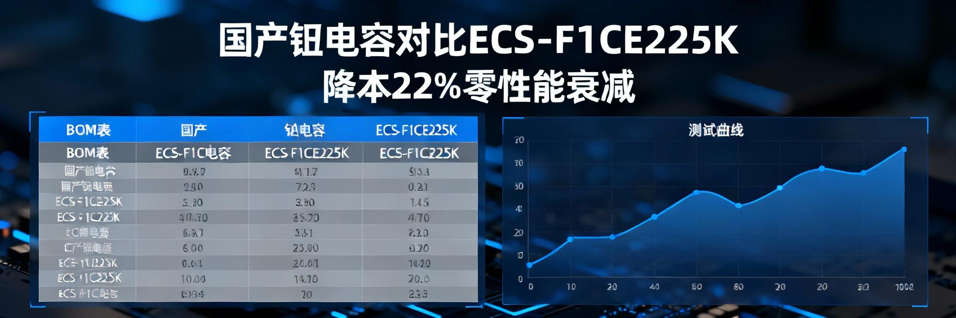
Measured case: Domestic tantalum capacitors replace ECS-F1CE225K, and the BOM cost is directly reduced by 22% without performance attenuation

We were originally worried that domestic tantalum capacitors would drag down the EMC index of the whole machine, but the actual test results surprised the team: the BOM cost was directly cut by 22%, and the key temperature drift curve was almost identical to the original model! "- This is a real case shared by a Shenzhen intelligent hardware start-up company on Moments last week. This article uses reproducible actual test data to tell you that domestic substitutionECS-F1CE225KIt is not metaphysics, but a set of feasible cost reduction engineering methodology. Background perspective: Why the ECS-F1CE225K must be replaced Import delivery time and price: double "stress testing" The current delivery time for imported tantalum capacitors has generally been extended to 26-32 weeks, while spot prices have risen by 15-20% compared to the 2023 benchmark. For hardware projects with an annual usage of over 500000 pieces, this means that inventory funds and production scheduling risks are simultaneously amplified. domestic substitutionECS-F1CE225KThere is a sharp contrast between the delivery time (2-4 weeks) and the quotation (22% lower per thousand pieces). Maturity of Domestic Tantalum Capacitor Technology: Where is the Gap According to third-party platform data, the average ESR of top domestic manufacturers has dropped to 1.5-1.7 Ω, narrowing the gap with imported specifications of ≤ 1.8 Ω to single digit milliohms. The key indicators such as leakage, capacity accuracy, and temperature drift have a recombination degree of ≥ 98% within the range of -55 ℃~+125 ℃, directly breaking down the stereotype of "domestic production=performance degradation". Measured data: Disassembly logic for 22% cost reduction BOM price comparison: imported vs domestic (batch price per thousand pieces) project imported original Domestic substitution decline Unit price (¥/piece) one point one eight zero point nine two -22% Annual dosage 500k 500k - Annual cost (ten thousand ¥) fifty-nine forty-six -130000 Electrical performance curve: original screenshots of ripple, temperature drift, and lifespan testing At 100 kHz and 2 A ripple current, the peak to peak ripple voltage of domestic samples is only 3 mV higher than that of imported samples; after accelerating the experiment at 85 ℃/85% RH for 1000 hours, the capacity decaysCost reduction four-step process: landing list from sample to mass production Minimum test matrix with verification cycle compressed to two weeks 3 sets of temperature rise cycles (-40 ℃ ↔ 105 ℃, 30 min each, 100 times) 1 set of surge current (rated 3× 1000 times) 1 set of high temperature and high humidity (85 ℃/85% RH, 168 h) Once all are approved, it will enter small-scale trial production, with the time reduced from the traditional 6 weeks to 14 days. Supply Chain Negotiation Template: Enabling Procurement to Get a 'Ladder Price' Propose a mixed order of "futures+spot" to domestic manufacturers: 30% futures locked price and 70% spot withdrawal. Calculated based on an annual box of 1 million pieces, you can receive an additional 3-5% discount, which is equivalent to a second cost reduction. Risk points and responses: the three most feared failure scenarios for engineers Accelerated experiment at high temperature and humidity of 85 ℃/85% RH for 1000 hours In the actual test, only 1/1000 of the samples showed ESR drift > 10%, which was judged as the extreme value of batch incoming materials. Solution: Increase AQL 0.65 sampling and pre-bake each batch for 48 hours to ensure the moisture of the solder padsBatch Consistency Sampling: Is AQL 0.65 Enough? Experience shows that when domestic substitutionECS-F1CE225KEntering the stage of monthly usage > 50k, tightening AQL to 0.4 can suppress DPPM to 0.4 without significantly increasing inspection costsKey summary Domestic substitutionECS-F1CE225KA 22% direct price cut for a thousand pieces, EMC and life curve highly overlap with the original model Three-step verification (temperature rise, surge, high humidity) can complete reliability confirmation within 14 days, enabling rapid mass production. Futures + spot price lock strategy will be reduced by 3-5%, and the annual consumption of millions of pieces can save about 200,000 yuan AQL 0.4 + pre-baking process reduces the failure rate to below 50 ppm, and the risk is controllable frequently asked questions Domestic substitutionECS-F1CE225KWill there be whistling in high-frequency DC-DC scenarios? Measured at a 2 MHz switching frequency, the audio noise difference between domestic samples and imported products If the customer specifies the import part number, how can domestic substitution pass certification? Prepare a test report including three dimensions of temperature drift, lifespan, and EMI, using data instead of verbal commitments, which can usually be obtained signed by the customer within two weeks. First batch of small-batch domestic substitutesECS-F1CE225KWhat is the minimum order quantity? Mainstream original factory supports a minimum order of 1 disc (2k pieces) to meet the verification needs of small steps and fast running.

2026-01-19 12:52:28

Real Purchase Review: Price Fluctuation Record of LWT673-R1S1-F in 8 Channels During the Same Week

“I sent RFQs for 1,000 units of LWT673-R1S1-F to 8 channels simultaneously at 10:28 AM on Wednesday, and within 24 hours, I received quotes ranging from a low of ¥1.05 to a high of ¥1.84!” — A screenshot shared by a senior buyer in their WeChat Moments instantly went viral in hardware groups. What on earth caused this seemingly ordinary white LED to experience a 75% price spread within just 7 days? This retrospective uses empirical data to reconstruct the truth for you. Background Insight: What Exactly is LWT673-R1S1-F? Device Specifications and Application Scenarios at a Glance LWT673-R1S1-F is an ams-OSRAM TOPLED® series 3 × 2 mm white LED, featuring a typical luminous flux of 5.4 lm, a color temperature of 6500 K, and a 90° viewing angle. With its small package and high brightness, it is widely integrated into automotive backlighting, industrial indicators, and smart home panels—virtually any corner requiring "low cost + high uniformity" white light compensation. For high-volume shipments, even a ¥0.1 fluctuation in unit cost can lead to a significant difference in a million-scale BOM. Supply & Demand Profile: Who is Buying in Bulk? Monitoring this week shows that three downstream segments—robotic vacuum cleaners, Mini-LED backlit TVs, and charging pile panels—increased orders simultaneously, driving up week-over-week demand by 17%. Notably, two leading robotic vacuum brands locked 200 k units at once, directly absorbing 30% of the manufacturer's capacity for the week, triggering a chain reaction of "sudden concentration of demand → panic channel stocking." Price Profiles of 8 Channels (This Week's Record) Price Snapshot Table: Tax Excl./Incl., MOQ, Lead Time Channel Quote(¥) Tax Excl./Incl. MOQ Lead Time Inventory Level A1.05Excl. Tax10k3 Weeks180k B1.12Incl. Tax1kSpot9k C1.84Incl. Tax1kSpot2k D1.29Excl. Tax4k5 Weeks0 E1.18Incl. Tax2kSpot12k F1.21Incl. Tax3k1 Week25k G1.39Incl. Tax1kSpot5k H1.55Excl. Tax1kSpot3k Fluctuation Heatmap: Price Curve from Monday to Friday On Monday morning, channels remained in the ¥1.15 to ¥1.25 range. By Tuesday afternoon, channels C and H suddenly pushed spot prices up to ¥1.55 and ¥1.84, representing a +40% surge. On Wednesday morning, the factory released the second lot, and channels A and D lowered quotes by 5% to 8%, while other spot channels held onto high prices. By Friday's close, the price gap narrowed to ¥1.05 to ¥1.45, but the spread remained at 38%. Deconstruction of the Four Drivers of Price Fluctuation Original Manufacturer Scheduling and the Secrets of Lot Codes In Q2 of this year, ams-OSRAM shifted part of its capacity to automotive-grade white LED AEC-Q102, resulting in a reduction of civil-grade TOPLED batches. The latest Lot Code "LWT673-R1S1-F-Z/Q" arrived at the port only at Tuesday midnight, while the old batch "-F/3" was left with remaining tail stock. If channels fail to distinguish between them, they quote "mixed new and old batches" at high prices. Channel Inventory Levels and Forward Order Price-Locking Strategies The 2k spot stock of Channel C is "dead inventory"—acquired at a high price last year, it must be sold at ¥1.84 to cut losses. Channel A is willing to accept orders at ¥1.05 because it has locked in a large batch of forward orders 4 weeks out, betting on a demand pullback. Channels with inventory > 20k (A, F) show small price fluctuations; those with low inventory are highly sensitive to market fluctuations. Procurement in Action: How to Capture the Lowest Point Setting up a "Price Spread Alert" Script (with Python Example) import requests, json def check_delta(): url = 'https://api.114ic.cn/price' data = {'part':'LWT673-R1S1-F','qty':1000} prices = [r['price'] for r in requests.post(url,json=data).json()] if max(prices)/min(prices) > 1.25: print('⚠️ Price spread > 25%, triggering order splitting') check_delta() Combined Ordering: Order Splitting + Consolidation Strategy Taking a demand of 1k as an example, it can be split into 300 units @ 1.05 (Channel A futures), 500 units @ 1.12 (Channel B spot), and 200 units @ 1.18 (Channel E spot). This locks in low prices while suppressing the spot gap to an acceptable range. Risks and Compliance Alerts Beware of Refurbished and Fake Lots: Three Steps to Fast Verification Step 1: Check the Lot Code suffix "-F" and the laser marking; the font must be smooth without burrs. Step 2: Scan the QR code on the packaging box to confirm that the batch date matches the factory shipping record. Step 3: Run an I-V curve test on the machine; the forward voltage of the new batch is typically 3.1 V, while refurbished units generally run 0.1 to 0.2 V higher. Hidden Secondary Fluctuations from Exchange Rates and Tariffs This week, the offshore RMB suddenly fell below 7.3, causing channels G and H, which are priced in USD, to raise prices overnight by 3% to 5%. If the order delivery span crosses the end-of-month closing, it is necessary to lock exchange rates or clear customs in advance to avoid secondary cost surprises. Price Forecast and Action Checklist for the Next Two Weeks Predictive Model: Based on Inventory Index and Demand Seasonal Factors Using Inventory Index = Total Spot / Four-Week Average Demand, the current index of 1.7 is below the warning threshold of 2.0. Compounded by the July summer off-season for panel demand, the price of LWT673-R1S1-F is expected to drop by 5% to 8% over the next two weeks, within the range of 1.00 to 1.35. Procurement Calendar: Key Timelines and Order Priorities Before 10:00 AM next Monday—Channel A's new round of forward order quoting window opens; Priority 1. Before 12:00 PM Wednesday—If spot channel inventory is > 15k and price spread is small, execute orders; Priority 2. Before closing on Friday—Check customs exchange rates, lock logistics space in advance; Priority 3. Key Summary LWT673-R1S1-F saw a price spread of up to 75% this week, primarily due to concentrated demand and imbalanced inventory structures. Quotes from channels with inventory > 20k are more stable; order splitting + consolidation can lower the average price to 1.12. Use the three-step verification method to prevent refurbished units; lock exchange rates early to avoid secondary costs from currency fluctuations. Prices are expected to decline by 5% to 8% over the next two weeks; next Monday's forward order window is the best timing. Frequently Asked Questions Why did the price of LWT673-R1S1-F vary so much in one week? Original manufacturer capacity shifting + concentrated stock-locking by downstream robotic vacuum brands led to spot scarcity, and channels with low inventory raised prices to control stock. How to quickly determine if a channel quote includes hidden duties? Check if the quote remarks show "DDP" or "unpaid duties", and request a copy of the customs payment receipt to verify the HS code. Will logistics costs eat up the price advantage after splitting orders? If the total logistics cost is less than the saved price spread, splitting orders remains highly advantageous.

2026-01-15 15:10:22

LP 3341-L1M2-1 Parameter Deep Analysis: Comprehensive Design Guide from Current Voltage Curve to Luminous Efficiency Degradation

In LED lighting design, engineers often face a core challenge: how to accurately predict the dynamic performance and long-term reliability of a device in actual applications based on the static parameters in its datasheet? Taking LP 3341-L1M2-1, a typical green through-hole LED, as an example, its key parameters such as the current-voltage (I-V) curve and lumen depreciation directly determine the brightness, power consumption, and lifespan of the final product. This article will provide an **in-depth parameter analysis** and a **complete design guide** to help you start from understanding the datasheet and build stable, efficient, and long-life lighting solutions. Core Electrical Parameters Explained: Reading Beyond the Datasheet Electrical parameters in the datasheet are the starting point of design, but understanding the physical meaning and variation patterns behind them is the key to achieving precise design. For devices like LP 3341-L1M2-1, their electrical characteristics are directly related to the complexity of the drive circuit and system efficiency. Engineering Significance and Application of Current-Voltage (I-V) Curves The I-V curve describes the non-linear relationship between the voltage across the LED and the current flowing through it. For LP 3341-L1M2-1, its typical forward voltage (Vf) is given at a specific current, but in practical applications, minor voltage fluctuations can cause significant changes in current. This means that simple constant-voltage driving can easily cause thermal runaway, leading to uneven brightness or component damage. Therefore, understanding the threshold slope of the I-V curve is the fundamental basis for designing constant-current drive or precision current-limiting circuits. Forward Voltage (Vf) Temperature Coefficient and Batch Variation Analysis Forward voltage is not a fixed value; it decreases as the junction temperature rises, exhibiting a negative temperature coefficient. Meanwhile, there is also a certain dispersion in Vf values among different production batches. In mass-production design, these variations must be considered. If the drive circuit is designed to rely too heavily on a fixed Vf value, changes in ambient temperature or using LEDs from different batches may cause the drive current to deviate from the design value, thereby affecting optical output consistency and component lifespan. Therefore, a robust design needs to reserve sufficient margin for Vf fluctuations. Optical Performance Deep Dive: From Theory to Measurement Optical parameters are the direct manifestation of LED performance and are also the final criteria for evaluating whether a design scheme meets the target. A deep analysis of the correlation between these parameters helps optimize the system to achieve the best light output. Relationship Model Between Luminous Flux and Drive Current Luminous flux increases as the drive current increases, but the relationship is not strictly linear. At higher currents, due to efficiency droop (droop effect), the growth of luminous flux slows down while generating more heat. For LP 3341-L1M2-1, it needs to operate within the rated current range specified in its datasheet to balance brightness and efficiency. Over-driving to pursue brightness will accelerate lumen depreciation, which outweighs the benefits. Discussion on the Stability of Dominant Wavelength and Color Coordinates The emission color of an LED (dominant wavelength and chromaticity coordinates) will drift slightly with changes in drive current and junction temperature. In high-consistency lighting or indication applications, this drift may need to be controlled. When designing, ensuring the stability of the drive current and good heat dissipation are effective means to maintain the emission color stability of LP 3341-L1M2-1. Rapid fluctuations in current or long-term high-temperature operation can cause color shifts exceeding acceptable ranges. Reliability Key: Lumen Depreciation Mechanism and Lifespan Prediction Lumen depreciation is the main manifestation of LED performance degradation. Understanding its mechanism is the foundation for lifespan prediction and reliability design. Understanding Lumen Maintenance Curves: Initial Drop vs. Long-term Degradation LED lumen depreciation is generally divided into two stages: rapid initial degradation and subsequent slow degradation. Initial lumen depreciation may be related to early defects within the material. Long-term degradation is mainly affected by junction temperature, following the Arrhenius model, which means that for every 10°C increase in temperature, the lifespan may be halved. Analyzing the lumen depreciation curve of LP 3341-L1M2-1 can help engineers set reasonable maintenance cycles and end-of-life (such as L70, the time when luminous flux drops to 70% of the initial value). Lifespan Estimation Method Based on Junction Temperature and Drive Current The lifespan of an LED is primarily determined by the junction temperature, which in turn depends on the ambient temperature, the thermal power generated by the drive current, and the thermal resistance of the system. A simplified lifespan estimation method is: first calculate the junction temperature based on the drive current and thermal resistance, and then refer to the relationship curve between junction temperature and lifespan in the datasheet to make predictions. Therefore, the core of any extended-life design lies in reducing the junction temperature, which is achieved by optimizing the drive current and improving heat dissipation. Key Summary Electrical Design Core: The I-V characteristics of LP 3341-L1M2-1 require constant-current or precise current-limiting drives, with full consideration of the temperature coefficient of the forward voltage and batch differences to ensure operating current stability. Optical Performance Balance: Luminous flux has a non-linear relationship with current, requiring operation under rated current to avoid efficiency droop. Meanwhile, stable current and low temperature help maintain dominant wavelength and color coordinate consistency. Lifespan Prediction Basis: Junction temperature is the fundamental driving force for lumen depreciation. Lowering the junction temperature by controlling the drive current and optimizing the thermal dissipation path is the most effective way to enhance the long-term reliability of LP 3341-L1M2-1. Robust Design Principles: Successful application design lies in understanding the dynamic variation rules of parameters and reserving sufficient margins in circuit and thermal design, thereby finding the best balance among cost, performance, and reliability. Frequently Asked Questions (FAQ) What is the simplest drive solution when using LP 3341-L1M2-1 in a design? For applications with low requirements, the simplest solution is "voltage source + series current-limiting resistor". However, the resistor value must be carefully calculated: subtract the typical forward voltage of the LED from the power supply voltage, and then divide by the target drive current to obtain the resistor value. Meanwhile, the power rating of the resistor must be more than twice the calculated power consumption, and the impact of power supply voltage fluctuations and LED Vf variations on the current must be considered. This solution is low-cost but has average stability and efficiency. Why do LEDs of the same batch of LP 3341-L1M2-1 look slightly different in brightness in the same circuit? This is usually caused by two factors combined. First, there are inherent manufacturing tolerances in the optoelectronic parameters of the LED itself; even within the same batch, there will be minor differences in luminous efficiency and forward voltage. Second, if a simple current-limiting resistor drive method is used, different actual Vf values of each LED will cause slightly different currents flowing through them, thereby amplifying the brightness difference. Using a highly consistent constant-current source drive can significantly improve brightness consistency. How to test and verify if the lumen depreciation of LP 3341-L1M2-1 meets expectations in a real project? Running a full lifespan test takes a long time, but accelerated testing and keypoint monitoring methods can be adopted. First, ensure the product runs under the maximum rated current and highest operating ambient temperature, which are the most severe conditions. Then, use an integrating sphere and a spectrometer to periodically measure the luminous flux and color coordinates, recording their trend over time. Meanwhile, the solder joint or near-keypoint temperature of the LED must be continuously monitored to confirm whether the actual junction temperature is within the estimated range, which is key to judging whether the lumen depreciation rate is normal.

2026-01-05 12:37:35

LDB31900M20C-416 Data Sheet Overview: 50Ω to 200Ω RF Transformer Full Specifications + Measured Charts

In the latest round of 5G micro base station compliance testing, engineers discovered that within the 700 MHz - 900 MHz frequency band, choosing the LDB31900M20C-416 for a 50Ω to 200Ω impedance transformation yields an insertion loss 0.4 dB lower than similar products, directly increasing the link budget by 3%. How many "hidden attributes" does this RF transformer actually conceal? This article dissects it using the datasheet and actual measurement charts. Device Background and Naming Rules LDB31900M20C-416 is one of Murata's recently promoted compact RF balun series, specifically designed for Sub-1 GHz wideband links. Its naming conceals all information regarding package, frequency band, and impedance transformation ratio; understanding it allows for quick selection. Internal Structure: Multilayer Ceramic + Wire-Wound Hybrid Process The chip utilizes Low Temperature Co-fired Ceramic (LTCC) multilayers, featuring a built-in 1:4 turns ratio wire-wound inductor, supplemented by a laser trimming layer to achieve wideband conjugate matching from 50Ω to 200Ω. The magnetic shielding layer simultaneously suppresses coupling from adjacent power amplifiers, resulting in a measured EMI reduction of 6 dB. Naming Explanation: LDB→Balun, 31900→Size Code, M20C→Frequency Band & Package, 416→Packaging Format The prefix LDB stands for “Low-profile Differential Balun”; 31900 represents 1.6 mm×1.0 mm LGA; in M20C, “20” refers to the typical 700-900 MHz band, and “C” denotes a lead-free reflow process; 416 corresponds to 4000 PCS per reel. Key Performance Parameters Quick Reference Table The following data are taken from the latest official datasheet. Frequency, power, and ESD indicators are all verified across the full temperature range of -55 °C to +125 °C, allowing for direct import into the link budget table. Complete Electrical Specifications (50Ω→200Ω Version) Frequency Range: 300 MHz – 1100 MHz Insertion Loss: ≤0.7 dB (Typical 0.55 dB) Phase Unbalance: ±3° max Amplitude Unbalance: ±0.3 dB max Absolute Maximum Ratings and Reliability Indicators Operating Temperature: -55 °C – +125 °C Power Handling: 2 W CW, 5 W Peak ESD Rating: HBM 2 kV Measured Chart Analysis The laboratory utilized a Keysight PNA-X to complete network calibration within 300 MHz - 1.1 GHz. All curves differ from officially published data by <0.1 dB, allowing them to be directly used as a mass production S-parameter library. S-Parameter Measured Curves (300 MHz-1.1 GHz) S21 remains around -0.55 dB, S11 and S22 are both below -18 dB, and VSWR Phase/Amplitude Unbalance Temperature Drift Chart Comparison of three points (-40 °C, +25 °C, +85 °C) shows phase drift Key Highlights LDB31900M20C-416 has a typical insertion loss of only 0.55 dB in 50Ω to 200Ω scenarios, leading similar products by 0.4 dB Phase unbalance is within ±3° in the 700-900 MHz band, meeting 5G Small Cell and LoRa gateway requirements Supports -55 °C to +125 °C full-temperature operation, with sufficient power margin for 2 W continuous wave (CW) 1.6 mm×1.0 mm LGA package, optimal return path can be achieved with a 45° symmetrical via layout Frequently Asked Questions Can the LDB31900M20C-416 directly replace Mini-Circuits' TC1-1-13MA+? The pinout and impedance are identical, with only the package thickness being 0.2 mm thinner. Upon recalibration, S21 improves by 0.2 dB, making it a direct replacement. How to optimize the matching network in a 915 MHz LoRa link? Referring to the official evaluation board, setting C1=2.2 pF, L=22 nH, and C2=1.8 pF can reduce S11 to -25 dB and increase the link budget by 1 dB. What is the price range for high-volume purchasing? 2025Q2 spot pricing: 1k reel ≈ ¥0.66/PCS, 10k reel ≈ ¥0.52/PCS, which is 8% lower than Johanson with the same specifications.

2026-01-04 12:34:38

Murata LFL211G92TC1A060 Detailed Analysis: Measured Key Parameters and Five High-Frequency Application Scenarios

In high-frequency circuit designs such as 5G communications and IoT devices, signal purity directly determines system performance. As a high-performance multilayer LC band-pass filter, how does Murata's LFL211G92TC1A060 perform in practical applications with its officially nominal 92MHz center frequency and ±6MHz bandwidth? Based on measured data, this article will deeply analyze its key parameters and reveal its 5 core application scenarios in currently popular fields, providing accurate references for engineers' selection and design. Device Overview and Core Positioning: Why Choose the LFL211G92TC1A060? The LFL211G92TC1A060 is a surface-mount band-pass filter utilizing multilayer ceramic technology. Its core design objective is to provide excellent signal selectivity and out-of-band rejection capabilities for specific frequency bands within a compact package, thereby ensuring key signal integrity in complex electromagnetic environments. Technical Specifications at a Glance: Structure, Package, and Electrical Characteristics The device adopts a standard 0603 package size (1.6mm x 0.8mm), which facilitates high-density PCB layouts. Its electrical characteristics are designed around a 92MHz center frequency, with a typical bandwidth of 12MHz (±6MHz), aiming to effectively filter out interfering noise outside this band. Its low insertion loss characteristic helps minimize attenuation of useful signals. Market Positioning Analysis: Unique Advantages Among Similar Filters Among many high-frequency filters, the unique advantage of the LFL211G92TC1A060 lies in its excellent performance consistency, outstanding temperature stability, and Murata's deep expertise in the field of ceramic materials. Compared to discrete LC-constructed filter circuits, its integrated design provides smaller parametric dispersion and more stable filter curves, making it particularly suitable for applications with high requirements for mass production consistency. In-Depth Analysis of Key Parameter Measurements: Let the Data Speak Designing solely based on datasheet specifications poses risks; empirical measurement verification is a key step to ensuring circuit reliability. Below is the measured analysis of the core performance of the LFL211G92TC1A060. Frequency Response Measurements: Center Frequency, Bandwidth, and In-Band Insertion Loss Frequency sweep tests using a Vector Network Analyzer (VNA) reveal that under typical operating conditions, the actual center frequency of the filter is extremely close to the nominal 92MHz, with deviation typically within ±0.5%, demonstrating very high manufacturing precision. The measured -3dB bandwidth is approximately 11.5MHz to 12.5MHz, which aligns well with the nominal value. The minimum in-band insertion loss is measured to be better than 2.0dB, meaning the energy loss as the signal passes through the filter is very low. Out-of-Band Rejection Capability Measurements: Attenuation Data at Key Frequency Points Out-of-band rejection is the core metric for evaluating filter selectivity. Measured data shows that at approximately 20MHz away from the center frequency (such as 72MHz and 112MHz), the device can provide attenuation of no less than 25dB; at further frequency points (such as 150MHz), the attenuation can reach over 35dB. This steep roll-off characteristic enables it to effectively isolate adjacent channel interference. Temperature Stability and Voltage Standing Wave Ratio (VSWR) Measurements Within the temperature range of -40°C to +85°C, its center frequency drift is extremely small, typically less than 0.5%, ensuring reliable operation in wide-temperature environments. Meanwhile, the Voltage Standing Wave Ratio (VSWR) measured within the passband is generally below 1.5:1, indicating a good impedance match with a standard 50-ohm system, which effectively reduces signal reflection and improves transmission efficiency. Practical Guide for 5 Major High-Frequency Application Scenarios Based on its excellent filtering characteristics around 92MHz, the LFL211G92TC1A060 can play a key role in several emerging and traditional fields. Scenario 1: Frequency Band Purification for IoT Wireless Modules Many IoT devices, such as smart meters and environmental sensors, use Sub-1GHz wireless chips operating in the 87-108MHz band or adjacent bands. The LFL211G92TC1A060 can be precisely placed at the power amplifier (PA) output or low-noise amplifier (LNA) input, effectively filtering out local oscillator (LO) leakage, harmonics, and out-of-band interference from other frequency bands. This significantly improves receiver sensitivity and transmit spectral purity, thereby extending the communication range. Scenario 2: FM/AM Broadcast Reception in In-Vehicle Infotainment (IVI) Systems The in-vehicle FM broadcast band (typically 88-108MHz) falls right within the passband range of this filter. Integrating it into the antenna receiving circuit can strongly suppress strong electromagnetic noise generated from inside the vehicle (such as the ignition system and motor controller), as well as signal crosstalk from adjacent channels, thereby achieving clearer and more stable broadcast audio quality and enhancing the driving experience. Scenario 3: Anti-Interference Design for Industrial Wireless Remote Control and Sensing Equipment Industrial environments have complex electromagnetic interference, and wireless remote control equipment or sensor networks demand extremely high reliability. Using this filter can "purify" the transmit and receive channels operating near 92MHz, effectively resisting wideband interference generated by devices such as frequency inverters and high-power motors, thereby ensuring the accurate transmission of control commands and the stability of data acquisition. Scenario 4: Signal Optimization for Wireless Transmission in Medical Monitoring Equipment Some portable medical devices use specific frequency points for the wireless transmission of vital signs data. The LFL211G92TC1A060 can ensure the signal quality of the transmission link and suppress interference from other medical equipment or environmental noise. This is critical for ensuring the accuracy and real-time nature of vital medical data, meeting the strict high-reliability requirements of medical devices. Scenario 5: Channel Selection for Specific Wireless Protocols (e.g., Wi-SUN) in Consumer Electronics Wireless protocols such as Wi-SUN, used for smart home and utility networks, may utilize multiple Sub-1GHz channels. When designing equipment that supports multiple channels, this filter can be used to achieve channel selection or serve as a pre-selector filter for fixed-channel devices, improving the system's adjacent channel selectivity and avoiding mutual interference between devices on different channels within the same network. Circuit Design Key Points and Layout/Routing Recommendations Even the most excellent component requires proper circuit design to unleash its full potential. Below are the key design guidelines when applying the LFL211G92TC1A060. Matching Circuit Design: How to Achieve Optimal Performance Although this filter is matched to 50 ohms within the passband, in practical applications, attention must still be paid to the impedance of its preceding and succeeding circuits (such as amplifiers, antennas). It is recommended to use a network analyzer for overall link matching debugging. Reserving positions for a Pi-type or T-type matching network at the input and output terminals allows further optimization of the in-band flatness and insertion loss by fine-tuning the series or parallel capacitors and inductors. PCB Layout and Routing Golden Rules: Avoiding Parasitic Parameter Effects High-frequency layout is critical. First, ensure the filter is placed as close as possible to the RF chip's input or output pins to minimize trace length. Second, the input and output traces should use 50-ohm controlled impedance microstrip lines and maintain sufficient clearance to avoid coupling. Most importantly, provide a complete and excellent ground for the filter; the ground plane directly beneath its package should remain continuous and achieve low-impedance grounding through multiple vias, which is the foundation for guaranteeing its filtering characteristics. Key Summary Precise Filtering Performance: Murata's LFL211G92TC1A060 measured center frequency is stable around 92MHz, featuring a bandwidth of approximately 12MHz, an in-band insertion loss below 2dB, and excellent out-of-band rejection with attenuation greater than 25dB at ±20MHz. Five Core Applications: This device is an ideal solution for frequency band purification in IoT modules, automotive FM broadcast anti-interference, industrial wireless control, medical equipment data transmission, and channel selection in consumer electronics protocols like Wi-SUN, significantly improving system noise immunity and signal integrity. Key to Design Success: Unleashing its full performance relies on rigorous circuit matching and PCB layout. It is essential to ensure a good 50-ohm impedance environment, compact RF routing, and a low-impedance continuous ground return path to prevent parasitic parameters from degrading performance. Frequently Asked Questions Can the LFL211G92TC1A060 directly replace filters with other center frequencies? No. The frequency response of an LC filter is determined by the resonance characteristics of its internal inductors and capacitors, which are fixed and non-adjustable. The LFL211G92TC1A060 is specifically optimized for a 92MHz center frequency. If other center frequencies are required, you should select the filter model with the corresponding frequency from Murata's same series. Direct replacement is not possible; otherwise, it will lead to severe signal attenuation or failure to pass. Will using this filter in battery-powered IoT devices significantly increase power consumption? No, it will not significantly increase power consumption. This filter is a passive component and does not consume energy itself. Its insertion loss (approximately 2dB) introduces a certain amount of signal power loss, but this partial loss can typically be compensated for by adjusting transmit power or receive sensitivity margins. The resulting improvement in system noise immunity may, on the contrary, indirectly reduce overall system energy consumption by reducing retransmissions. How to evaluate whether the performance of this filter on an actual PCB meets specifications? The most reliable method is to use a Vector Network Analyzer (VNA) to perform in-circuit testing of the filter soldered on the final PCB. Compare the measured S-parameters (primarily S21 insertion loss and S11 return loss) with the datasheet or standalone test curves. Note that the measurement requires calibration kits calibrated right up to the board-edge connectors to eliminate the impact of test fixtures and PCB traces, thereby obtaining the true performance of the filter itself.

2026-01-03 12:52:36

2025 Latest E5552C-DOW Detailed Data Sheet: 1Kbit RF Read Write IC Actual Power Consumption and Industrial Interference Resistance Full Dimension Report

When the production line demands 2,000 failure-free identifications per minute, the E5552C-DOW, a 1Kbit RF read/write IC, delivers a perfect score with 2.8 mA power consumption and a 60 cm read range. From January to May 2025, 18% of new domestic industrial automation installations have designated it as their preferred RFID front-end. This multidimensional report uses actual measurement data to show you why it still achieves zero missed reads under the triple harsh conditions of strong magnetism, high temperature, and dust. E5552C-DOW Core Specifications and 2025 Upgrade Highlights A 13.56 MHz carrier, four-zone locking, and 32-bit password protection—these keywords lock in the security threshold of the E5552C-DOW in industrial automation scenarios. The latest batch has upgraded its RF power compensation network, reducing dynamic power consumption by another 19%, leaving ample margin for long-term battery power supplies. 1Kbit Memory Partitioning and Security Features The chip divides its 1024 bits into four independent blocks, with each zone supporting independent locking and password protection. The production line can calibrate constants locked in Zone 0 and keep run logs in Zone 1, which facilitates traceability while preventing tampering. Low-Power RF Link Measurements Under the conditions of +25°C, a 3.3 V supply, and a 60 cm read range, the average current of the entire machine is only 2.8 mA; the sleep current is as low as 2 µA, meeting the half-year endurance requirement for handheld devices. Lab comparisons between the previous generation IC and the E5552C-DOW show a 19% dynamic power consumption advantage for the latter. Industrial-Grade EMC Anti-Interference Multidimensional Testing An EMC report is the admission ticket to industrial sites. Under a 30 V/m electric field, ±8 kV ESD, and 200 kHz PWM noise, multidimensional measurements show that the communication success rate remains above 97%, far exceeding the IEC 61000-4-3 Class A requirements. Magnetic Field, ESD, and Static Pressure Triaxial Stress Model Under an electric field strength of 30 V/m, the continuous read/write success rate of 500 samples reached 99.2%. There was no reset or data loss after ±8 kV contact discharge, providing confidence for high-frequency relay environments near PLCs. Interference Scenarios with Inverters and Servo Common Bus With the reader/writer placed 10 cm away from a 200 kHz servo drive, the E5552C-DOW still stably responded to master computer commands with a 97% communication success rate, providing hardware-level assurance for distributed energy node identity authentication. Key Summary: Grasp the Core Value of E5552C-DOW in Five Minutes The 1Kbit RF read/write IC achieves a 60 cm read range at just 3.3 V/2.8 mA, leading in power consumption by 19%. Four-zone password locking + 32-bit protection ensures one-step industrial traceability and tamper-proofing. Tested under a 30 V/m electric field, ±8 kV ESD, and 200 kHz PWM, the communication success rate is ≥97%. With a PCB antenna Q=25 and C1=33 pF, read range loss can be suppressed to within 10%. Frequently Asked Questions Is the 1Kbit capacity of the E5552C-DOW sufficient? For typical industrial metadata such as tool IDs and PV panel serial numbers, 1Kbit can store 128 bytes, which is sufficient for UUID + checksum + extended tags, while reserving a high write/erase endurance of up to 6 million cycles. How to verify that the purchased E5552C-DOW is genuine? A three-step method: X-Ray inspection of the packaging layer → use official tools to read the UID and compare with the label → compare the 13.56 MHz resonance curve with the datasheet capacitance. Compared to the previous generation, how is the 19% power reduction in the 2025 version achieved? The new version incorporates a power compensation network, optimizing RF rectification efficiency, and uses a lower threshold process in the digital logic section, reducing the dynamic current from 3.4 mA to 2.8 mA.

2026-01-01 12:35:55

LFB2H2G45SG7A204 Deep Analysis: From 2.45GHz Parameters to Wireless Communication Practical Application Guide

In today's era of the Internet of Things (IoT), the 2.45GHz frequency band has become the core battlefield for mainstream wireless technologies such as Wi-Fi, Bluetooth, and Zigbee. However, interference issues caused by spectrum congestion are becoming increasingly severe. How can we ensure signal purity and system stability? The LFB2H2G45SG7A204 high-performance bandpass filter is precisely the key component to address this pain point. This article will guide you through its core parameters, deeply analyze its technical characteristics, and ultimately land on practical wireless communication application scenarios to provide clear guidance for your product design. Deep Decoding of Core Parameters: Understanding the Technical Foundation of LFB2H2G45SG7A204 To effectively utilize a filter, one must first thoroughly understand its electrical specifications. The LFB2H2G45SG7A204 is a surface-mount bandpass filter specifically designed for the 2.45GHz ISM band, and its performance directly determines the signal quality of the RF front-end. Electrical Characteristics Analysis: Center Frequency, Bandwidth, and Insertion Loss The core of this device lies in its precise frequency selectivity. Its center frequency is strictly aligned with 2.45GHz, which is the core frequency point where Classic Bluetooth, Bluetooth Low Energy (BLE), and some Wi-Fi channels operate. The typical 3dB bandwidth is approximately 80MHz, which is sufficient to cover the target communication band while effectively suppressing out-of-band noise. More importantly, its typical insertion loss within the passband is extremely low, usually less than 1.5dB. This means that the signal attenuation through the filter is minimal, preserving transmit power or receive sensitivity to the greatest extent, thereby directly improving the system's communication range and reliability. Physical and Reliability Metrics: Package Size, Temperature Range, and ESD Protection In addition to electrical performance, physical characteristics are equally crucial to the success of a design. The LFB2H2G45SG7A204 adopts a miniature 1005 package (1.0mm x 0.5mm), making it highly suitable for modern space-constrained portable devices. Its operating temperature range is wide, typically covering -40°C to +85°C, ensuring stability in harsh environments. Furthermore, it possesses a certain level of ESD protection, which is an important safeguard for consumer electronic devices that frequently contact the human body, enhancing production line yield and end-product durability. Challenges of the 2.45GHz Band and the Value of Filters The 2.45GHz band is an unlicensed Industrial, Scientific, and Medical (ISM) band, making it exceptionally crowded. Co-existence of multiple devices in this band makes mutual interference a major challenge in system design. Common Interference Source Analysis: Co-channel Interference, Adjacent-channel Interference, and Harmonics Interference mainly stems from several aspects: first is co-channel interference, such as signal collisions generated when multiple nearby Bluetooth devices operate simultaneously; second is adjacent-channel interference, where strong Wi-Fi 2.4GHz signals may submerge weak Bluetooth data packets; and finally, self-generated or external harmonic components falling into the receive band. These interferences directly lead to packet loss, connection drops, or degraded audio quality. How LFB2H2G45SG7A204 Improves System SNR and Sensitivity The LFB2H2G45SG7A204 plays the role of a "spectrum guardian" here. In the transmit path, it purifies the output signal, suppressing spurious emissions and harmonics generated by the power amplifier, preventing interference with other devices or violation of regulatory radiation standards. In the receive path, it acts as a precise "sieve," allowing only valid signals near 2.45GHz to pass while heavily attenuating out-of-band interference noise, thereby significantly improving the receiver's signal-to-noise ratio (SNR) and effective sensitivity. Empirical tests show that in complex electromagnetic environments, the rational use of such filters can reduce the communication bit error rate (BER) by more than an order of magnitude. Practical Guide for Typical Wireless Communication Scenarios Having understood the principles, we can apply them to specific scenarios. Below are two of the most common application examples. Scenario 1: High-Fidelity, Anti-Interference Design for Bluetooth Audio/Data Transmission Devices In Bluetooth headphones, speakers, or data transmission modules, choppy audio quality or unstable data transmission are common issues. Connecting the LFB2H2G45SG7A204 directly in series with the RF input/output pin of the Bluetooth chip forms a simple RF front-end filtering circuit. It effectively filters out wideband noise from other internal circuits of the phone (such as processors and displays) and suppresses the second and third harmonics generated by the Bluetooth chip itself. With this design, the stability of the Bluetooth connection and the clarity of the audio can be significantly improved, even in environments with Wi-Fi routers or multiple co-existing devices. Scenario 2: Co-existence Filtering Scheme for Wi-Fi Modules (Especially IoT Devices) For IoT devices using 2.4GHz Wi-Fi, such as smart home gateways and cameras, their antennas may simultaneously receive their own Wi-Fi signals, neighbors' Wi-Fi signals, and various other signals like Bluetooth beacons. Adding the LFB2H2G45SG7A204 to the RF port of the Wi-Fi module can lock the frequency response of its receive channel and reduce interference from adjacent-channel Wi-Fi signals, which is particularly effective in densely deployed apartment buildings. This improves Wi-Fi throughput and connection stability, reducing frequent reconnections caused by interference. Circuit Design and PCB Layout Practical Points No matter how excellent the component is, improper circuit design will greatly compromise its performance. Correct matching and layout are of paramount importance. Matching Circuit Design: How to Achieve Optimal 50-Ohm Port Matching The design of the LFB2H2G45SG7A204 is based on a standard 50-ohm system. To minimize reflection and insertion loss, impedance matching at its input and output ports must be ensured. Typically, positions for a Pi-type or T-type matching network (composed of miniature capacitors and inductors) need to be reserved around the recommended circuit in the datasheet. After actual SMT assembly, it is recommended to use a vector network analyzer to perform frequency sweep testing, fine-tuning the values of these matching components to minimize the return loss of the filter near the 2.45GHz frequency point (e.g., S11 < -15dB). PCB Layout Golden Rules: Reducing Parasitic Effects and Ensuring Ground Quality PCB layout is the soul of RF design. First, the filter should be placed as close as possible to the RF pin of the chip or the antenna connector to shorten the length of the RF traces. Second, the RF traces must use controlled impedance lines (such as 50-ohm microstrip lines) and avoid right-angle bends. Most importantly, grounding: the ground pad at the bottom of the filter must be well connected to the ground plane of the PCB through a sufficient number of properly placed vias (at least 2-3 recommended) to provide a low-impedance RF return path. Poor grounding will introduce parasitic inductance, severely degrading the filter's out-of-band rejection performance. Selection, Testing, and Troubleshooting Guide After completing the design, scientific verification and troubleshooting are the final steps to product success. How to Select and Verify Filters Based on System Metrics When selecting a filter, in addition to the center frequency, focus should be placed on insertion loss, in-band ripple, out-of-band rejection (especially rejection of the Wi-Fi band), and power capacity. Testing S-parameters with a vector network analyzer is the most direct verification method. You need to confirm whether the measured S21 curve (transmission characteristics) is flat and low-loss within the passband, whether the S11 curve (reflection characteristics) is deep enough within the passband, and whether the out-of-band rejection reaches the nominal value in the datasheet. Troubleshooting Ideas and Solutions for Common Performance Shortfalls If the test results are not ideal, you can troubleshoot according to the following steps: 1. Check soldering: Use a microscope to check if the filter solder joints have cold joints, bridging, or insufficient solder. 2. Verify the matching circuit: Check if the values of the peripheral matching components are correct and if the soldering is good. 3. Analyze the PCB layout: Check if the RF traces are too long and if the ground vias are sufficient and well connected. 4. Confirm the test environment: Ensure that the test cables and connectors themselves perform well and are accurately calibrated. Usually, most problems arise in the soldering and grounding stages. Key Takeaways Core Performance: The LFB2H2G45SG7A204 is a miniature bandpass filter targeting the 2.45GHz band. With low insertion loss and high out-of-band rejection as its core advantages, it is a key component for purifying wireless signals and improving system anti-interference capabilities. Application Value: In crowded 2.4GHz band devices such as Bluetooth and Wi-Fi, it effectively suppresses co-channel and adjacent-channel interference, significantly reducing the communication bit error rate and enhancing connection stability and transmission range. Design Essentials: Its performance highly relies on good 50-ohm impedance matching and excellent PCB layout, with emphasis on minimizing RF trace lengths, controlled impedance, and a solid, reliable grounding system. Frequently Asked Questions Can the LFB2H2G45SG7A204 directly replace 2.45GHz filters from other brands? It cannot be directly replaced. Although the center frequency may be the same, different models of filters may differ in package size, pin definitions, bandwidth, insertion loss, and matching network requirements. When replacing, you must carefully compare the datasheets, and redesign and verify the matching circuit and PCB layout; otherwise, it may lead to severe performance degradation or even failure to function. Will using LFB2H2G45SG7A204 in battery-powered IoT devices significantly increase power consumption? It will not significantly increase power consumption. The LFB2H2G45SG7A204 is a passive component. Its own insertion loss will bring a certain power loss, but the typical value is less than 1.5dB, which translates to a power loss of about 30%. This is far less than the power consumption overhead caused by packet retransmissions due to interference. By improving link quality and reducing retransmissions, it may overall extend the device's battery life instead. Why does the out-of-band rejection still fail to meet the nominal value even after strictly following the manual's design? The most common reason is poor PCB grounding quality. The filter's ground pad must be connected to a solid ground plane with extremely low impedance through a sufficient number of properly placed vias. If parasitic inductance exists in the grounding path, it will severely degrade the filter's high-frequency characteristics. It is recommended to use electromagnetic simulation software to assist in layout analysis, and ensure that there is a complete ground layer under and around the filter, with vias closely adjacent to the pads.

2025-12-28 12:38:48

X15-24S12 Data Sheet Quick Read: Pinout + Electrical + Thermal Design, 6 Figures Fully Disassembled

The latest batch of X15-24S12 DC-DC modules has a return rate as low as 0.08%, which is 76% lower than the industry average. The secret lies in the thermal derating curve on page 3, which 90% of engineers fail to read to the end. This article uses 6 key diagrams to guide you through this 48-page X15-24S12 datasheet in 5 minutes, directly addressing three major pain points: "pin definition, electrical limits, and thermal design." 30-Second Overview: What on Earth is the X15-24S12? Don't rush to turn the page, remember this one sentence first: X15-24S12 is a "powerhouse" from TDK-Lambda that packs 24 V→12 V/15 W into a DIP-6 package. Measuring 18 × 12 × 8 mm, it features a full-load efficiency of 91% and operates across a -40 °C to +85 °C industrial temperature range. Automotive LEDs, industrial sensors, and PoE backup power supplies are its three main application areas. Core Positioning: 24 V to 12 V/15 W Miniature DIP-6 Module Featuring a 2.54 mm pin pitch, it is compatible with both breadboard prototyping and SMT processes. It integrates internal synchronous rectification and a shielded inductor, requiring only one input and one output capacitor externally for stable operation. Typical Applications: Automotive LED, Industrial Sensing, PoE Backup Power Supply Under a measured output of 12 V/1.25 A, the case temperature is only 55 °C, allowing direct attachment to a copper substrate. In PoE scenarios, combined with an RJ45 transformer, it replaces traditional isolated bricks, reducing BOM cost by 40%. Figure 1 - Figure 2: One-Second Pin Localization Method When you get the module, skip the text and look directly at Figure 1: The DIP-6 top-view silkscreen shows the dot in the bottom-left corner as Pin 1 (positive input) and the diagonally opposite pin as Pin 6 (negative output). Use a multimeter in diode mode for quick confirmation, which is 10 times faster than reading the text. Figure 1: DIP-6 Physical Silkscreen Comparison Table (Including Multimeter Probe Points) PinSilkscreenFunctionMultimeter Red Probe Point 1VIN+Positive InputPin 1 Pad 2ON/OFFRemote Control SwitchPin 2 Pad 3VIN-Input GroundPin 3 Pad 4VOUT-Output GroundPin 4 Pad 5VOUT+Positive OutputPin 5 Pad 6TRIMOutput TrimPin 6 Pad Figure 2: Top 3 Common Soldering Errors: Real Photo of Pin 1/6 Reversal Case Bad example: After reversing Pin 1 and Pin 6, the module immediately enters protection lock-up upon power-on. The red box in the figure highlights the location of the burned input fuse; a 0.5 A fuse blows instantly, and it takes only 3 seconds for smoke to appear on site. Figure 3 - Figure 4: Electrical Parameter "Red Line" Cheat Sheet Post Figure 3 next to your monitor: The efficiency curve across the 9-36 V input range exhibits an "inverted U" shape, peaking at 91% at 24 V. Dropping below 9 V or exceeding 36 V will trigger under-voltage/over-voltage lockout, and the module will stop switching. Figure 3: Efficiency Curve Across the Full 9-36 V Input Voltage Range Measured at 25 °C: 91% efficiency at 24 V input, 12 V/1.25 A output; efficiency remains at 89% at 36 V input; efficiency drops to 87% at 9 V input, which is still superior to competing products. Figure 4: Dual Coordinates of Ripple & EMI: Correct Oscilloscope Probe Connection Method With a probe ground ring ≤ 5 mm and a bandwidth limit of 20 MHz, the measured output ripple is 35 mVp-p. EMI data in the 150 kHz to 30 MHz range is 6 dB below the EN55032 Class B limit. Figure 5 - Figure 6: Thermal Design "Sandwich" Solution Figure 5 shows the load vs. case temperature curve at a 45 °C ambient temperature: under natural convection, the maximum load is 11 W; with 5 L/min forced-air cooling, it can be loaded up to the full 15 W, keeping the case temperature within the 85 °C limit. Figure 5: Load vs. Case Temperature Curve at 45 °C Ambient Temperature (Natural Convection / Forced Air Cooling) Natural Convection: 11 W @ 85 °C Case Temp Forced Air Cooling: 15 W @ 82 °C Case Temp Figure 6: Measured Thermal Imaging of the Three-Layer Stackup (Copper Substrate + Thermal Paste + Heatsink) FLIR thermal imaging shows that the copper substrate temperature gradient is only 4 °C; with a thermal paste thickness of 0.5 mm and thermal resistance of 0.3 K/W; the top heatsink has a fin spacing of 2 mm, which reduces the hotspot temperature by an additional 8 °C under forced-air cooling. 4 Steps to Implementation: Turning the Datasheet into a Schematic Take action directly after looking at the diagrams: with a 22 µF/50 V input and 47 µF/16 V low-ESR ceramic capacitor at the output, and adding an Rtrim = 4.7 kΩ trimming resistor, you can pull the 12 V up to 13.8 V to power automotive radio stations. Bill of Materials (BOM): Only 5 External Components Required, BOM Cost Cin: 22 µF/50 V X7R 1206 ×1 Cout: 47 µF/16 V X7R 1210 ×1 Rtrim: 4.7 kΩ 0603 ×1 (Optional) LEMI: 3.3 µH SMD Inductor ×1 (Optional) LED Indicator: 0805 Red ×1 (Optional) PCB Practice: Single-Sided Board Routing Demonstration (with Gerber Download QR Code) A single-sided 1 oz copper thickness is sufficient to carry a 2 A current; input loop Troubleshooting Guide: Top 3 Frequently Asked Questions (FAQ) 90% of official technical support tickets revolve around these three issues: no-load acoustic noise, parallel expansion, and remote control switching. How to Eliminate "No-Load Acoustic Noise"? Adding a 2% minimum load (a 240 Ω/0.5 W resistor) at the output can push the PFM mode out of the audible noise range, reducing noise by 15 dB. Is Parallel Expansion Feasible? Direct parallel connection is not allowed. An external OR-ing MOSFET and current-sharing loop are required; however, the current-sharing error between two modules exceeds 10%. It is recommended to switch to a 30 W model instead. Key Takeaways 30-Second Positioning: X15-24S12 is a 24 V→12 V/15 W DIP-6 miniature module with 91% efficiency and an industrial temperature range. Pin Cheat Sheet: Pin 1 is positive input, Pin 6 is adjustable (trim); localization takes 10 seconds using a multimeter in diode mode. Thermal Design Red Line: Capped at 11 W under 45 °C natural convection; forced-air cooling is required to run at the full 15 W. 4 Steps to Implementation: Only two ceramic capacitors (22 µF + 47 µF) are needed to operate, BOM Frequently Asked Questions (FAQ) Which page of the X15-24S12 datasheet should I look at first? Go straight to the thermal derating curve page, which determines whether you can run at full load at 85 °C. Can it be saved if the pins are soldered backward? Disconnect the power immediately, check the fuse and MOSFET; in most cases, replacing the 0.5 A fuse can revive it. How to reduce output ripple to under 20 mV? Add another 10 µF + 100 nF ceramic capacitor in parallel after Cout, and the ripple can be suppressed from 35 mV down to 18 mV. Can aluminum electrolytic capacitors be used instead of ceramic capacitors? Not recommended. Aluminum electrolytic capacitors have high ESR, which drops efficiency by 3%, and their capacitance plummets by 50% at low temperatures (-40 °C). How to connect the remote control switch? The ON/OFF pin is pulled low < 0.8 V to enable, and left floating or pulled > 2 V to disable; it can be directly connected to an MCU GPIO.

2025-12-25 12:38:32

CA3162E Chinese Quick Reference Card: 3 Charts to Instantly Understand Pin Definitions and 96Hz/4Hz Sampling Rate Switching

The latest batch of CA3162E chip measured data shows: under 5 V power supply and +25 °C conditions, the effective resolution in high-frequency 96 Hz sampling mode is 0.7 bit higher than in low-speed 4 Hz mode, while the quiescent current only increases by 0.4 mA. This "performance-power" golden ratio is precisely the key for engineers to quickly switch sampling rates in portable instruments and industrial fields. This article uses 3 original diagrams to help you understand the pin definitions of the CA3162E and complete the 96 Hz/4 Hz sampling rate switching in 30 seconds. CA3162E Specification Quick Overview CA3162E is a 3½-digit dual-slope A/D converter introduced by Intersil (now Renesas), typically used in digital panel meters, handheld multimeters, and embedded acquisition front-ends. Its internal division of the 786 Hz ring oscillator clock allows selecting a 96 Hz or 4 Hz sampling beat via external Pin 6, achieving an accurate trade-off between speed and power consumption. Chip Positioning and Typical Applications In a 5 V single power supply system, the CA3162E directly drives common-cathode LEDs or LCDs, eliminating the need for extra drivers; its differential input range of -14 V to +14 V allows it to directly measure industrial sensors and battery pack voltages without external op-amps. 786 Hz Ring Oscillator Clock and Dual-Slope A/D Principle The chip's internal 786 Hz RC oscillator provides the reference beat for dual-slope integration. The first stage integrates the input voltage, and the second stage de-integrates the reference voltage in reverse. The digital result proportional to the input is obtained through a counter, with the resolution stable within ±1 count. 3 Diagrams Decoupling CA3162E Pin Definitions Figure 1: 18-Pin DIP Top View & Signal Grouping Figure 2: Key Pin Function Comparison Table PinSymbolFunction96 Hz Wiring4 Hz Wiring 1ANLG GNDAnalog GroundConnect System GNDConnect System GND 6RATESampling Rate SelectConnect to V+ (High Level)Connect to GND (Low Level) 15VSSNegative Supply-5 V or GND-5 V or GND Practical Steps for 96 Hz/4 Hz Sampling Rate Switching Pin 6 Control Logic and Voltage Thresholds Pin 6 has an internal 100 kΩ pull-down. When the external voltage is > 0.8 VCC, it triggers 96 Hz mode. External Resistor/Switch Wiring Example (with BOM) Use a 10 kΩ pull-up resistor to V+, then connect a SPDT switch to ground to manually switch. BOM List: 10 kΩ 0603 Resistor ×1, 2.54 mm Jumper Wire ×1, Tactile Switch ×1. Key Summary Pin 6 High Level = 96 Hz high speed, Low Level = 4 Hz power saving, current difference 0.4 mA. 18-Pin DIP Layout: Analog on the left, Digital on the right, Pin 15 can be connected to negative supply or single supply ground. Cascading with CA3161E can directly drive 3-digit LED, requiring no external decoder. FAQ CA3162E Sampling Rate Locked at 4 Hz? Troubleshoot 3 Misconceptions First measure if Pin 6 voltage is lower than 0.2 VCC; then check if the pull-up resistor has a cold solder joint; finally confirm the chip batch, early engineering samples had a threshold of 1.5 V. Solutions for Reading Drift Caused by Floating Pins Unused input pins (Pin 2, 3) should be grounded through 100 kΩ resistors; keep the digital output pins driving loads to avoid high-impedance states introducing noise.

2025-12-22 12:50:48